26. Stokes' Theorem

a. The Theorem

1. Statement

Stokes' Theorem with a Single Boundary Curve
Let $S$ be a nice surface in $\mathbb{R}^3$ with a nice properly oriented boundary, $\partial S$ , and let $\vec{F}$ be a nice vector field on $S$ . Then $\iint_S \vec{\nabla}\times\vec{F}\cdot d\vec{S} =\oint_{\partial S} \vec{F}\cdot d\vec{s}$ If the boundary of the surface is a single closed curve, then the boundary must be traversed counterclockwise as seen from the tip of the normal vector to the surface.

Notice that the relative orientation of the surface and it boundary is crucial. If you reverse the direction of the normal to the surface, or if you reverse the direction the boundary curve is traversed (but not both) then the LHS and RHS of the theorem will not be equal, they will differ by a minus sign.

The vector field $\vec{F}$ is nice if it has continuous first partial derivatives. Similarly, the surface, $S,$ and its boundary, $\partial S,$ are nice if they are defined by parametric functions with continuous first partial derivatives.

Show Hand

In words, Stokes' theorem says the flux of the curl of a vector field $\vec{F}$ over a surface $S$ is equal to the circulation of $\vec{F}$ around the boundary curve $\partial S$ . This makes sense in that $\vec{\nabla}\times\vec{F}\cdot \vec{N}$ measures the rotation of the stuff around the $\vec{N}$ -axis. So the left side is the total rotation on the surface while the right side is the net rotation around the boundary.

Notice that on the left hand side (LHS) of the theorem, we are integrating the curl of the vector field, $\vec{\nabla}\times\vec{F}$ (and not just $\vec{F}$ ). Since $\vec{\nabla}\times\vec{F}$ is a vector field and we are integrating it over a surface, we need to dot it into the vector differential of surface area, $d\vec{S}=\vec{N}\,du\,dv$ . Similarly, on the right hand side (RHS) of the theorem, we are integrating $\vec{F}$ (and not its curl). Again, since $\vec{F}$ is a vector field and we are integrating it over the boundary curve, we need to dot it into the vector differential of arc length, $d\vec{s}=\vec{v}\,dt$ .

It is recommended that you first compute $\vec{\nabla}\times\vec{F}$ in rectangular coordinates, and then convert it to the coordinates needed for the surface integral. Computing $\vec{\nabla}\times\vec{F}$ in other coordinate systems is beyond the scope of this course.

Recall that Green's theorem related an integral over a region in the plane to an integral over its boundary curve. Stokes' theorem is a generalization of Green's theorem to $3$ dimensions in which the region in the plane is deformed into a surface in $3$ -dimentional space. In fact, Green's theorem is technically a special case of Stoke's theorem, namely for a surface which happens to lie in a plane. See the page on the 2D Stokes' Theorem.

Stokes' Theorem is usually applied to a surface whose boundary is a single closed curve. So that is where we start:

Compute $\displaystyle \iint_C \vec{\nabla}\times\vec{F}\cdot d\vec{S}$ for the vector field $\vec{F}=(-yz,xz,z^2)$ over the cone, $C$ , given by $z=\sqrt{x^2+y^2}$ for $z\le 3$ oriented down and out.

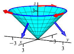
We use Stokes' Theorem to convert the surface integral over the cone into a line integral around the boundary of the cone which is a circle. $\iint_C \vec{\nabla}\times\vec{F}\cdot d\vec{S} =\oint_{\partial C} \vec{F}\cdot d\vec{s}$

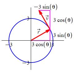
The circle may be parametrized by $\vec r(\theta)=(3\cos\theta,3\sin\theta,3)$ . So its velocity is $\vec v=\langle -3\sin\theta,3\cos\theta,0\rangle$ . If we look at this in the first quadrant where $\sin\theta \ge 0$ and $\cos\theta \ge 0$ , then $v_x \le 0$ and $v_y \ge 0$ . So $\vec v$ points counterclockwise, which is backwards! We need $\vec v$ clockwise. So we reverse $\vec v$ : $\text{Reverse:}\qquad\vec v=\langle 3\sin\theta,-3\cos\theta,0\rangle$

On the curve, the vector field $\vec{F}=(-yz,xz,z^2)$ becomes: $\left.\vec{F}\right|_{R(r,\theta)} =\langle -9\sin\theta,9\cos\theta,9\rangle$ So the line integral is: $\begin{aligned} \oint_{\partial S} \vec{F}\cdot d\vec{s} &=\int_0^{2\pi} \vec{F}\cdot\vec v\,d\theta \\ &=\int_0^{2\pi} (-27\sin^2\theta-27\cos^2\theta+0)\,d\theta \\ &=-27(2\pi)=-54\pi \end {aligned}$

Check: Surface Integral Directly

To check, we compute the surface integral directly. We start by computing the curl of $\vec F$ : $\begin{aligned} \vec{\nabla}\times\vec{F} &=\begin{vmatrix} \hat\imath & \hat\jmath & \hat k \\ \partial_x & \partial_y & \partial_z \\ -yz & xz & z^2 \end{vmatrix} \\ &=\hat\imath(0-x)-\hat\jmath(0--y)+\hat k(z--z) \\ &=\langle -x,-y,2z\rangle \end {aligned}$ In cylindrical coordinates, the surface is $z=r$ . So a parametrization is: $\vec R(r,\theta)=\langle r\cos\theta,r\sin\theta,r\rangle$ On the surface, the curl of $\vec F$ is: $\left.\vec{\nabla}\times\vec{F}\right|_{R(r,\theta)} =\langle -r\cos\theta,-r\sin\theta,2r\rangle$ The normal is: $\begin{aligned} \vec N&=\vec e_r\times\vec e_\theta =\begin{vmatrix} \hat\imath & \hat\jmath & \hat k \\ \cos\theta & \sin\theta & 1 \\ -r\sin\theta & r\cos\theta & 0 \end{vmatrix} \\ &=\hat\imath(0-r\cos\theta)-\hat\jmath(0--r\sin\theta) +\hat k(r\cos^2\theta--r\sin^2\theta) \\ &=\langle -r\cos\theta,-r\sin\theta,r \rangle \end {aligned}$ This points up and in. (The $z$ -component is positive while the $x$ and $y$ components are negative in the first quadrant.) So we reverse the normal: $\text{Reverse:}\qquad\vec N=\langle r\cos\theta,r\sin\theta,-r\rangle$ Finally, we can compute the integral: $\begin{aligned} \iint_C \vec{\nabla}\times\vec{F}\cdot d\vec{S} &=\int_0^{2\pi}\int_0^3 \left.\vec{\nabla}\times\vec{F}\right|_{R(r,\theta)} \cdot \vec N\,dr\,d\theta \\ &=\int_0^{2\pi}\int_0^3 (-r^2\cos^2\theta-r^2\sin^2\theta-2r^2)\,dr\,d\theta \\ &=-\int_0^3 r^2\,dr \int_0^{2\pi} (1+2)\,d\theta \\ &=-\left[\dfrac{r^3}{3}\right]_0^3\left[\rule{0pt}{10pt}3\theta\right]_0^{2\pi} \\ &=-9(6\pi)=-54\pi \end {aligned}$

Both methods gave the same answer. This checks both computations and also verifies Stokes' Theorem for this function and surface. Notice how much easier the line integral was. This will not always be the case.

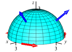
Use Stokes' Theorem to compute $\displaystyle \iint_H \vec{\nabla}\times\vec{F}\cdot d\vec{S}$ for the vector field $\vec{F}=(y,-x,-x^2-y^2)$ over the hemisphere, $H$ , given by $z=\sqrt{9-x^2-y^2}$ oriented up and out.

Answer

$\displaystyle \iint_H \vec{\nabla}\times\vec{F}\cdot d\vec{S} =\oint_{\partial H} \vec{F}\cdot d\vec{s}=-18\pi$

[×]

Solution

By Stokes' Theorem: $\iint_H \vec{\nabla}\times\vec{F}\cdot d\vec{S} =\oint_{\partial H} \vec{F}\cdot d\vec{s}$ The boundary is the circle of radius $3$ in the $xy$ -plane traversed counterclockwise, which may be parametrized as: $\vec r(\theta)=(3\cos\theta,3\sin\theta,0)$ The velocity is: $\vec v(\theta)=\langle -3\sin\theta,3\cos\theta,0\rangle$ which does point counterclockwise. On the circle, the vector field $\vec{F}=(y,-x,-x^2-y^2)$ becomes: $\begin{aligned} \left.\vec{F}\right|_{\vec r(\theta)} &=(3\sin\theta,-3\cos\theta,-9\cos^2\theta-9\sin^2\theta) \\ &=(3\sin\theta,-3\cos\theta,-9) \end {aligned}$ So the line integral is: $\begin{aligned} \oint_{\partial H} \vec{F}\cdot d\vec{s} &=\int_0^{2\pi} \vec{F}\cdot\vec v\,d\theta \\ &=\int_0^{2\pi} (-9\sin^2\theta-9\cos^2\theta+0)\,d\theta \\ &=-9(2\pi)=-18\pi \end {aligned}$

[×]

Check

We check by computing the surface integral directly. We start by computing the curl of $\vec F$ : $\begin{aligned} \vec{\nabla}\times\vec{F} &=\begin{vmatrix} \hat\imath & \hat\jmath & \hat k \\ \partial_x & \partial_y & \partial_z \\ y & -x & -x^2-y^2 \end{vmatrix} \\ &=\hat\imath(-2y)-\hat\jmath(-2x)+\hat k(-1-1) \\ &=\langle -2y,2x,-2\rangle \end {aligned}$ Since the surface is a hemisphere of radius $3$ , we parametrize starting with spherical coordinates and setting $\rho=3$ : $\vec R(\phi,\theta) =\langle 3\sin\phi\cos\theta,3\sin\phi\sin\theta,3\cos\phi\rangle$ On the surface, the curl of $\vec F$ is: $\left.\vec{\nabla}\times\vec{F}\right|_{R(\phi,\theta)} =\langle -6\sin\phi\sin\theta,6\sin\phi\cos\theta,-2\rangle$ The normal is: $\begin{aligned} \vec N&=\vec e_\phi\times\vec e_\theta =\begin{vmatrix} \hat\imath & \hat\jmath & \hat k \\ 3\cos\phi\cos\theta & 3\cos\phi\sin\theta & -3\sin\phi \\ -3\sin\phi\sin\theta & 3\sin\phi\cos\theta & 0 \end{vmatrix} \\ &=\hat\imath(--9\sin^2\phi\cos\theta)-\hat\jmath(-9\sin^2\phi\sin\theta) \\ &\quad+\hat k(9\sin\phi\cos\phi\cos^2\theta--9\sin\phi\cos\phi\sin^2\theta) \\ &=\langle 9\sin^2\phi\cos\theta,9\sin^2\phi\sin\theta,9\sin\phi\cos\phi\rangle \end {aligned}$ This points up and out as desired. Finally, we can compute the integral: $\begin{aligned} \iint_H \vec{\nabla}\times\vec{F}\cdot d\vec{S} &=\int_0^{2\pi}\int_0^{\pi/2} \left.\vec{\nabla}\times\vec{F}\right|_{R(r,\theta)} \cdot\vec N\,d\phi\,d\theta \\ &=\int_0^{2\pi}\int_0^{\pi/2} (-54\sin^3\phi\sin\theta\cos\theta+54\sin^3\phi\sin\theta\cos\theta \\ &\qquad-18\sin\phi\cos\phi)\,d\phi\,d\theta \\ &=-18\int_0^{2\pi}\int_0^{\pi/2}\sin\phi\cos\phi\,d\phi\,d\theta \\ &=-18(2\pi)\left[\dfrac{\sin^2\phi}{2}\right]_0^{\pi/2} =-18\pi \end {aligned}$

[×]

Remark

Both methods gave the same answer. This checks both computations and also verifies Stokes' Theorem for this function and surface. Notice how much easier the line integral was.

[×]

We have now verified Stokes' Theorem for a couple of functions and surfaces. We will verify it more later in this chapter and prove it still later.